The internet is awash with images generated by AI models like Midjourney, DALLE, and Stable Diffusion. But the images that accompany articles on it tend to be a bit same-y. Sci-fi themes, Blade Runner dystopian cities, anime. ‘Photorealistic’ images of women that come ready-airbrushed.

I wanted to experiment with generating some different looking images using a form of style transfer. I did this using textual inversion on Stable Diffusion.

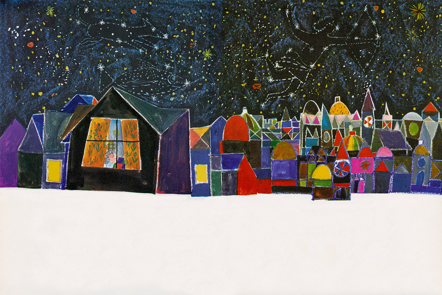
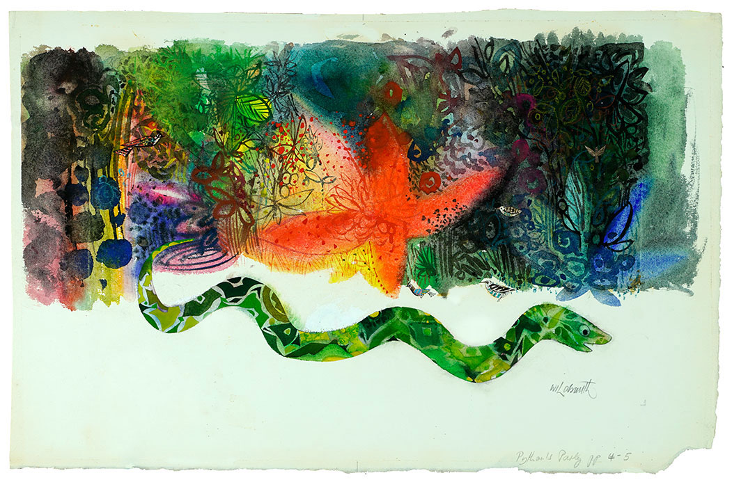
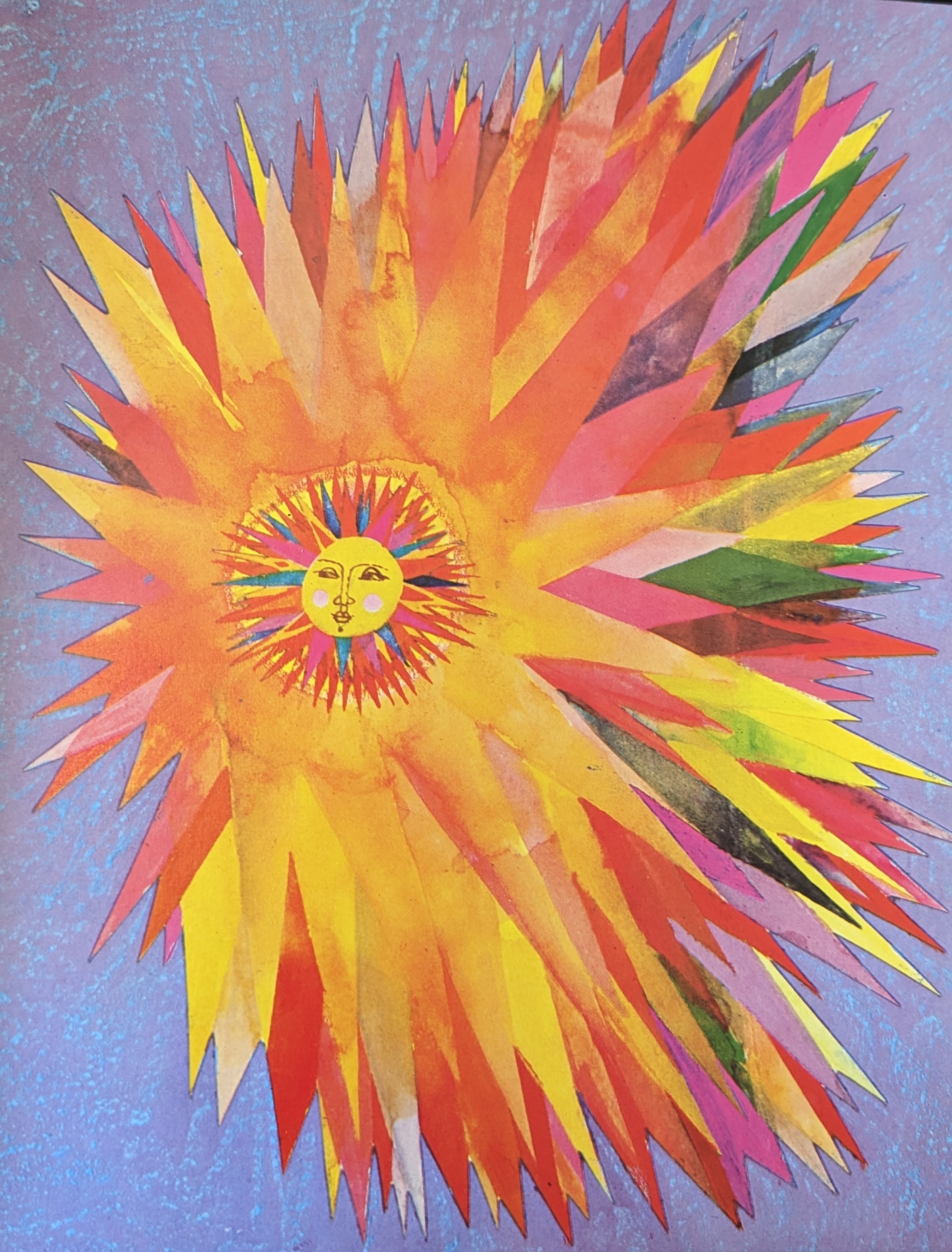
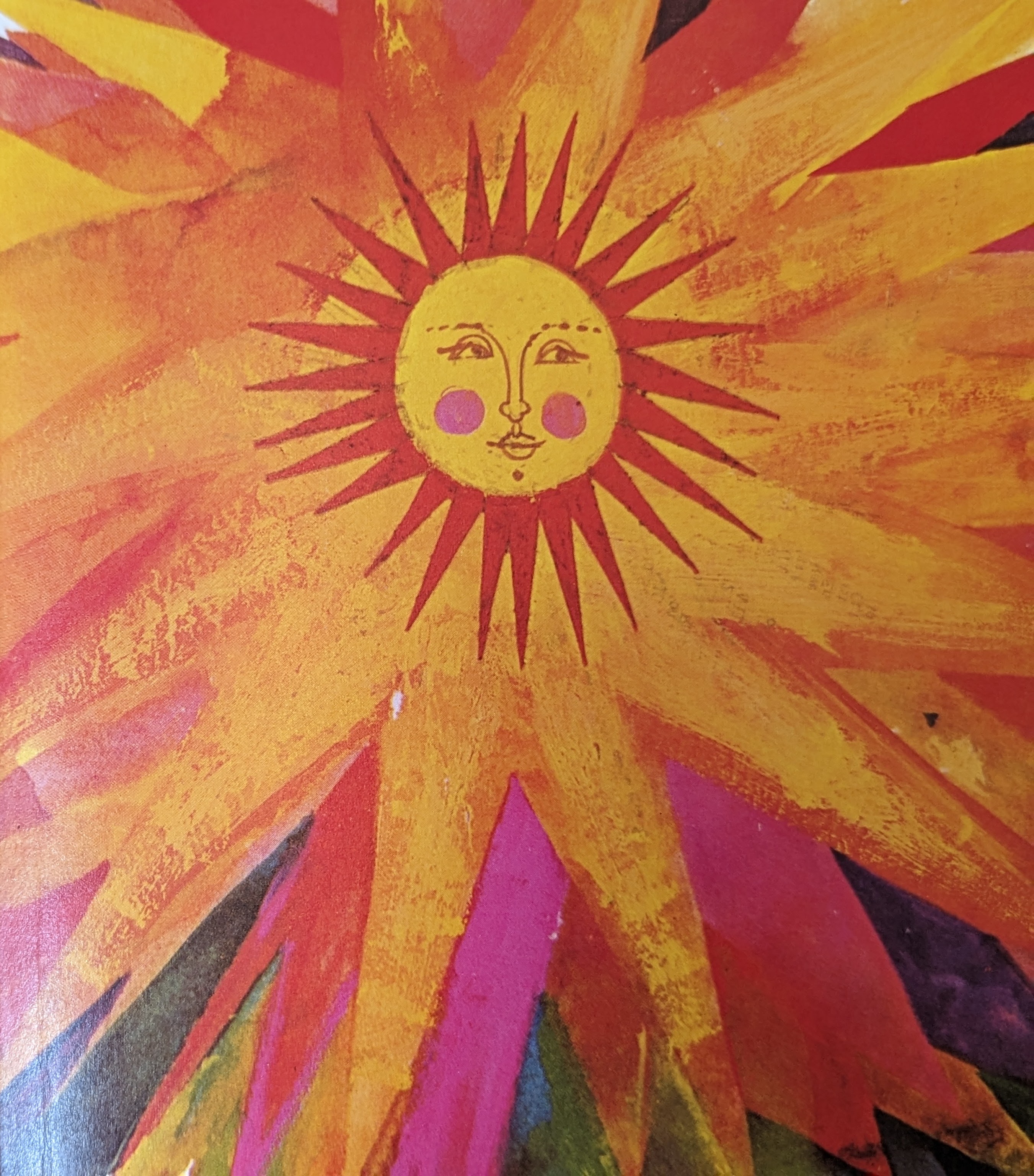
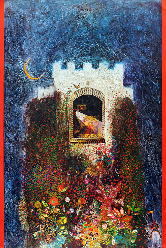
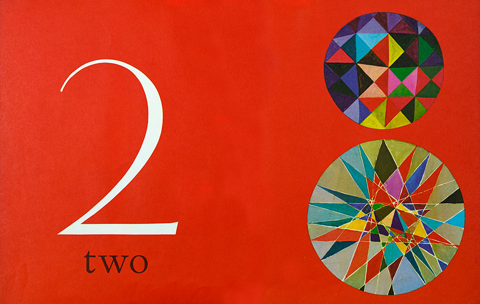
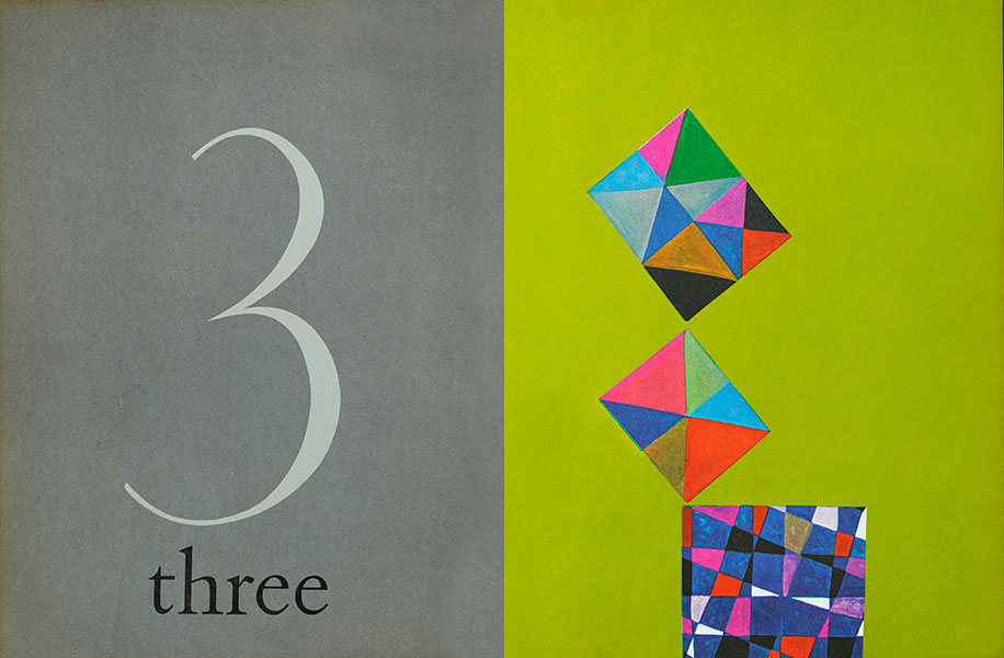
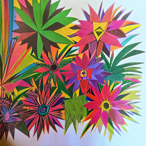
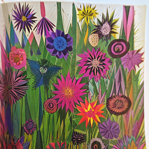
For this experiment, I wanted to push the model into recreating the textures, palettes and ornate style of children’s illustrator Brian Wildsmith. Wildsmith made books and posters using a range of media, from scratchy pen and ink to rich gauche. One of the most striking things about his work is the use of colour – fuscias, emerald greens, and frequent use of geometic patterns. I wanted to see how well the model would learn and apply these themes. This isn’t the simplest way to showcase style transfer, since Wildsmith’s style is very broad, spanning a lifetime of work.

In the post below, I take a deeper look at the textual inversion and its potential for use in adjusting generative AI trained on biased datasets. I’ll also dive into the mathematics of classifier-free guidance as it’s applied in this case.

Here are some examples of original Wildsmith:

Caveats

I don’t want to start throwing around derivative images without saying something about the relationship of style-transfer results to the original creations. Its clear that style-transfer results are dependent in a strong sense on the original artist, and right that the artist’s role be respected.

Can AI-generated images be art? My feeling is that on the one hand, simply grabbing the output image from a generative neural network isn’t producing a piece of art. However, these neural nets are tools, which can be used creatively, flexibly and imaginatively. Generative AI can be used to produce art, in an anaologous way to that in which artists create artwork with mixed media, photography, and other methods that differ from the traditonal paint and canvas.

There are certain characteristics of art that are essential to it. One is creativity. Secondly, art is, as I see it, essentially a form of human-to-human communication: the artist has some intention for the piece they are creating. This is why a sunset, however beautiful, is not art. So, it is possible for AI-generated media to be art, depending on the role played by the human in the process of their creation.

Given this understanding of the relationship between art and generative AI, we can address worries sometimes voiced about whether generative AI is going to replace artists.

Consider the minor scandal at the end of last year when a digital art prize was won by an entry generated by Midjourney. The winner gloated “Art is dead, dude. It’s over. A.I. won. Humans lost.” I don’t see how you can hold this view without knowing both very little about the technology and very little about art. Rather than being an adversary of art, generative AI is simply a new tool to be put to various uses.

However, this doesn’t mean that other professions won’t be heavily disrupted by generative AI. It seems inevitable that less creative image-generation, like stock photography, won’t end up being at least partially automated by generative AI.

Given that philosophical digression, let’s get back to the tech.

Textual inversion on a style

There is a lot of interest in fine-tuning large foundation models to make them applicible to custom domains. This isn’t simple to apply in practice, due amongst other things to the alarmingly named ‘catastrophic forgetting’. But there are reliable methods that can be used to add specific representational capacity to a pretrained model, such as textual inversion.

Textual inversion enables you to add a new pseudo-word to the embedding space of the model, representing a chosen image or style. The method effectively teaches the model the new word by examples.

Gal et al 2022 present textual inversion on text-to-image models. They suggest 3-5 images of an object is sufficient to embed it into the model. I started off with about 6 images in my training set, and then increased this considerably, first to 136 and ultimately to 318.

Data and setup

I used Automatic1111’s webui to train the textual inversion on Stable Diffusion v1.4.

My dataset was around 300 images I scanned from Brian Wildsmith books and found online. I named each file with a brief description of the content. The filenames are used in training to generate prompts of the form "a painting of [filewords] by [name]", where [filewords] come from the filename and [name] is the new pseudo-word.

Images were cropped to 512x512. One hurdle was how to programmatically crop the images in a way that preserved features of interest. Centre-cropping meant that the resulting models generated images missing the tops of heads. For speed, I used a feature of the webui to programatically crop based on detected focal point in combination with splitting large images into smaller, overlapping tiles, but this was not entirely satisfactory.

The work was done with permission of the Wildsmith family.

Results

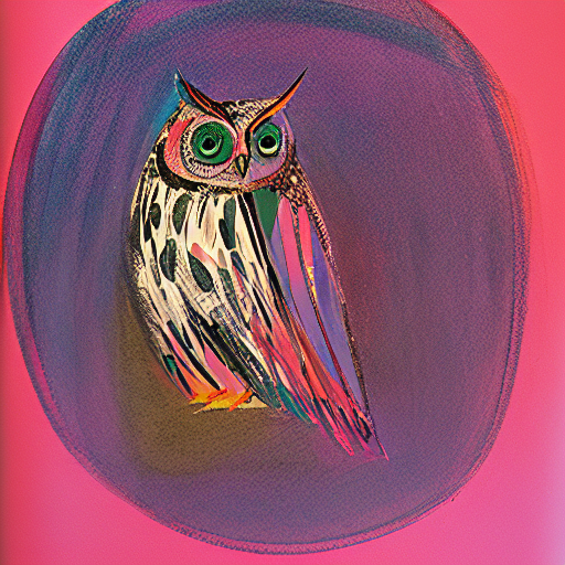
Here’s a couple of images that were generated randomly during training of the new embedding.

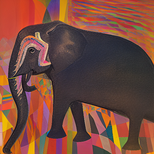
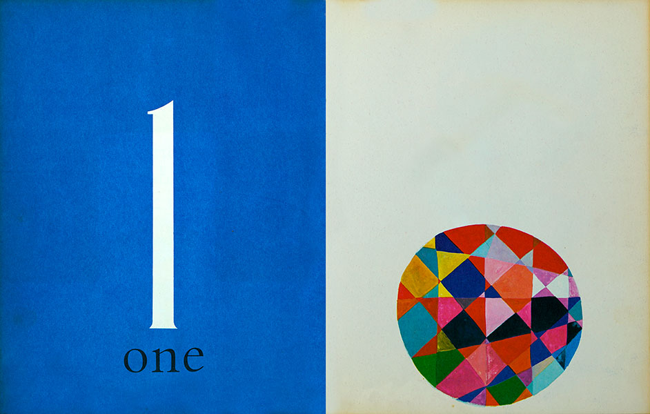
The geometric pattern in the background of the elephant is frequently generated by my model. It appears in the training set in some of Wildsmith’s illustrations of abstract shapes. For instance, from his counting book:

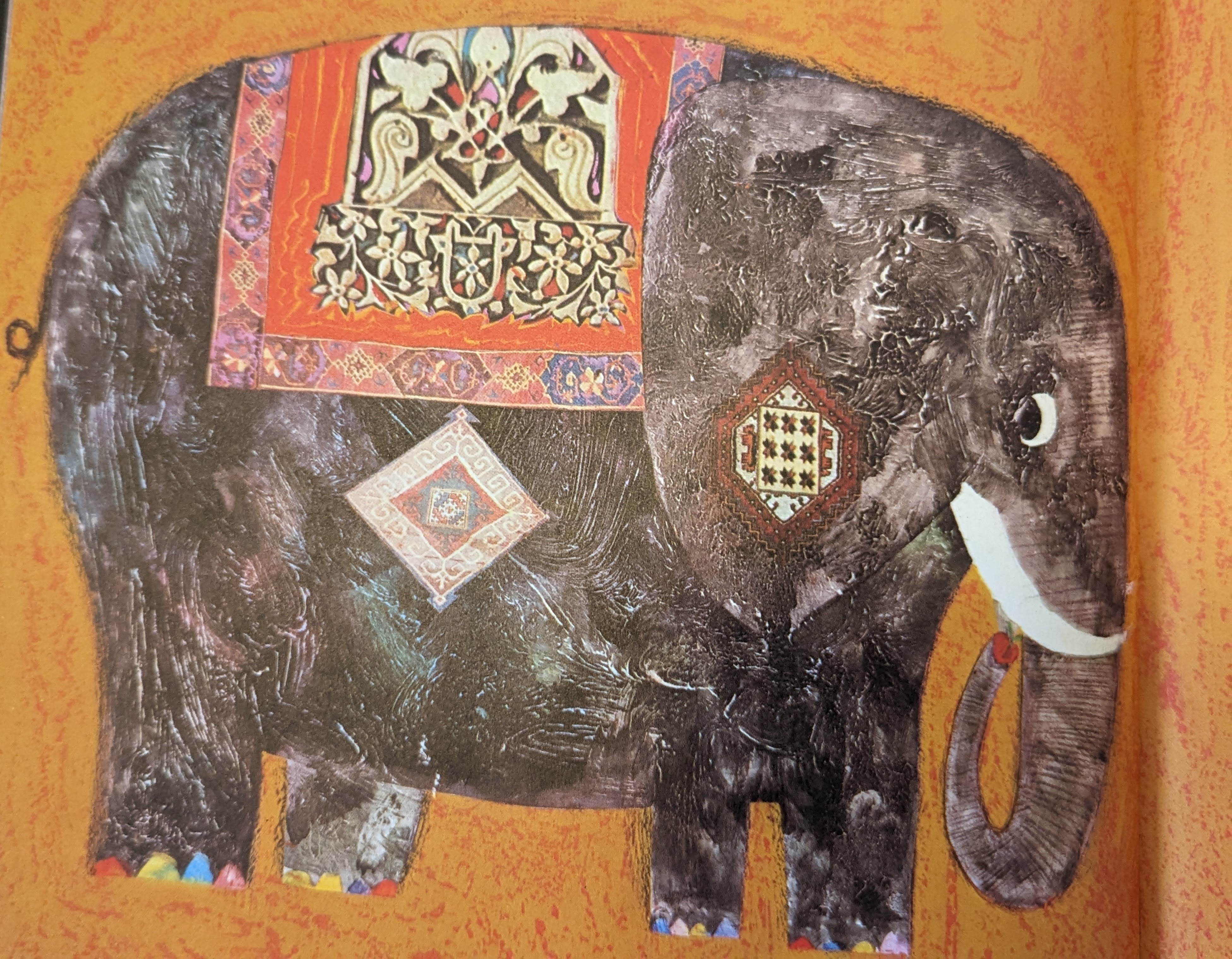
The decorative design on the elephant’s trunk does not appear in the training set, but was created by the model. The closest thing in the training set, in terms of content, is the following elephant with a decorative saddle. The generated image is clearly different and draws from different aspects of the Wildsmith style:

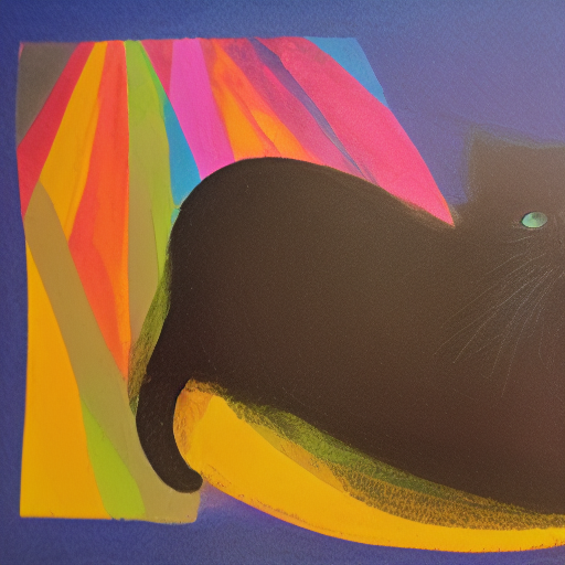
The following sets of examples were created using the same prompts, with embeddings using 1 and 16 vectors per token respectively, though different random seeds in each case. The version with 16 vectors per token captures more of the texture of the pencil and paintbrush strokes in the original images, as well as some unintended artefacts of the training data like page creases, photographic glare and shadows.

Results were generated with 20-80 sampling steps, and cfg_scale raised to 14 from the default 7. More on this parameter below. Theoretically higher cfg_scale values should force closer adherence to the prompt; I found they gave better looking results, although they tended to reproduce more of the unwanted artefacts too.

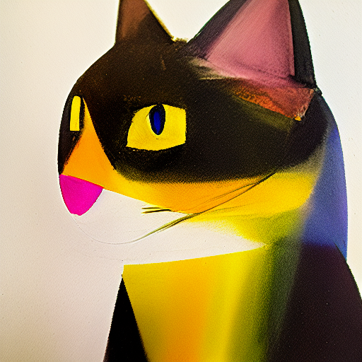
Using 16 vectors per token (sadly the cat image was a victim of the cropping issue):

Classifier-free guidance for style transfer

One parameter I experimented with was the value controlling classifier-free guidance. Classifier free guidance is a technique that can be applied at inference time to control the closeness with which the generated results adhere to the prompt. I wanted to understand what exactly classifier-free guidance is doing in the context of style transfer, both in terms of the mathematics and the visual results. In Automatic1111’s web UI, this parameter is cfg_scale.

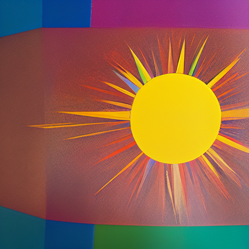
To show the effect of varying the classifier-free guidance scale, see the sequence of images below, for values ranging from 0 and 30 using a fixed seed. The model was prompted to draw a city of tents in the desert under a full moon, in Wildsmith’s style. It’s immediately noticable that while results for inital values in [0,1] don’t resemble the prompt, after this the model is gently exploring a set of similar points in the space.

This time, a house with a mountain range in the background. The image flickers between different placements of the house, leaving it out altogether for large classifier-free guidance scale values. Both of these quick experiments suggest that there is no benefit to tuning the classifier-free guidance scale beyond a certain point.

The method of classifier-free guidance developed from an earlier method, classifier guidance. This was introduced by Dhariwal and Nichol (2021) and was the technique that gave diffusion models the edge over GANs in image synthesis. I found Sander Dieleman blog post on guidance gave a careful motivation for the methods, and Lilian Weng’s blog post covered the maths. This post builds on their accounts by including concrete examples of varying the classifier free guidance values.

To see what classifier guidance does, let’s recap what exactly a conditional diffusion model like stable diffusion does. The trick to understanding the model is to see that what we are modeling – images – are sampled from a probability distribution $q(x)$, albeit an extremely complex one. Images are not noise; they have a structure, and this can be described by a distribution. We can also consider a noising process, called forward diffusion, in which we add incremental amounts of Gaussian noise to an image $x_{0}$ drawn from $q(x)$, giving us a sequence $x_{t}$ for $t\in[0, T]$ such that $x_{T}$ ends up being pure noise. If we had access to $q$, we could take a sample of this pure noise and apply the reverse of the diffusion process, denoising it back to content, by estimating $q(x_{t}\vert x_{t+1})$. This is not possible, however, since $q$ depends on the entire dataset of images and is therefore intractable to compute.

What we can do is to train a model that approximates these conditional probabilities $q(x_{t}\vert x_{t+1})$. Call this model $p_{\theta}(x_{t} \vert x_{t+1})$. Under certain assumptions, the distribution $p_{\theta}$ is a Gaussian. So now we can denoise images to get them back to noiselessness.

There is an additional hurdle: we would like to use a conditional diffusion model. This is to say, we want the denoising to be conditioned on some text prompt. We don’t just want our denoising process to reveal any image that looks like it came from the underlying distribution $q(x)$, but rather to reveal the image most closely aligned with a given text prompt, $y$. This means we are in fact dealing with the conditional probability $p_{\theta}(x_{t}\vert x_{t+1}, y)$, which can be also approximated by a Gaussian. In practice, diffusion models approximate $\nabla_{x}log(p_{\theta}(x \vert y))$, the ‘score function’ of the distribution, rather than the distribution itself.

Distribution $p_{\theta}$ gives rise to an associated denoising model $\epsilon_{\theta}(x_{t+1}, y)$, which predicts the noise at timestep $t$ given the prompt $y$ and the image $x_{t+1}$, which is equivalent to predicting the incrementally denoised image $x_{t}$.

So, how do we use the unconditional denoising model to generate images? This is explained in the following section.

Conditional reverse diffusion

Sampling from a conditional denoising model is possible given an additional classifier model trained on noisy versions of $x$ labeled with classes $y$. Dhariwal and Nichol, reason as follows: suppose first that we have a conditional Markovian noising process $\widehat{q}$, such that $\widehat{q}(y|x_{0})$ is a known label distribution for each sample. If this sounds familiar, it should: it’s exactly what you would get out of a softmax function at the end of a regular classifier model over classes $y$. Dhariwal and Nichol establish that $\widehat{q}(y|x_{t+1} \vert x_{t}) = \widehat{q}(y|x_{t+1} \vert x_{t}, y)$, which is just to say that the distribution doesn’t change whether or not it is conditioned on $y$. And they also prove, using the fact that $\widehat{q}(y|x_{0}) = q(y|x_{0})$, that $\widehat{q}(y|x_{t}) = q(y|x_{t})$. For the full derivation see Appendix H of the paper. Using these identities, and repeated applications of the multiplucation rule of probability, they can then establish that:

$\widehat{q}(x_{t} \vert x_{t+1}, y)$

$= \frac{\widehat{q}(x_{t}, x_{t+1}, y)}{\widehat{q}(x_{t+1}, y)}$

$= \frac{\widehat{q}(x_{t}, x_{t+1}, y)}{\widehat{q}(y \vert x_{t+1}) \widehat{q}(x_{t+1})}$

$ = \frac{\widehat{q}(x_{t} \vert x_{t+1}) \widehat{q}(y \vert x_{t}, x_{t+1}) \widehat{q}(x_{t+1})} {\widehat{q}(y \vert x_{t+1}) \widehat{q}(x_{t+1})}$

$= \frac{\widehat{q}(x_{t} \vert x_{t+1}) \widehat{q}(y \vert x_{t}) } {\widehat{q}(y \vert x_{t+1})}$

$= \frac{q(x_{t} \vert x_{t+1}) \widehat{q}(y \vert x_{t}) } {\widehat{q}(y \vert x_{t+1})}$ by previously established identity

$= Z q(x_{t} \vert x_{t+1}) \widehat{q}(y \vert x_{t})$, since $\widehat{q}(y \vert x_{t+1})$ does not depend on $x_t$, we can treat it as a constant $\frac{1}{Z}$.

Since $p_{\theta}(x_{t} \vert x_{t+1})$ approximates $q(x_{t} \vert x_{t+1})$, we have

$\widehat{q}(y \vert x_{t+1}, y ,x_{t}) \approx p_{\theta}(x_{t} \vert x_{t+1}) \widehat{q}(y \vert x_{t})$.

And we can, as mentioned in the previous paragraph, easily train a classifier to give us $\widehat{q}(y \vert x_{t})$. As we can therefore compute both factors of the left hand side, we can sample from the conditional reverse diffusion process $\widehat{q}(y \vert x_{t+1}, y ,x_{t})$.

OK, so that is an overview of how conditional diffusion models work. For the rest of the section we’ll follow the notational convention of suppressing the timestep annotations, and assume for each timestep $t$ a function $p_{\theta}(x\vert y) = p_{\theta}(x_{t}\vert x_{t+1}, y)$

The insight of classifier guidance is that we can modify the score function of the noise predictor $\epsilon_{\theta}$ in such a way that the denoised images produced at inference time are more closely aligned to the prompt. This works by introducing a scalar coefficient controlling one factor (the classifier term) of the score function.

In simple terms, in reverse conditional diffusion, we want to know how much the log-probability of an image $x$ given prompt $y$ changes when we change $x$, so we can iteratively move towards the $x$ that maximises this value. This is the gradient of the log-probability, $ \nabla_{x} log(p_{\theta}(x\vert y))$, which we introduced above as the score function.

We can apply Bayes rule, below, to rewrite the score function as follows:

Bayes rule entails that $p_{\theta}(x\vert y) = \frac{p_{\theta}(y\vert x).p_{\theta}(x)}{p_{\theta}(y)}$

Then, taking gradients w.r.t. $x$, and distributing the log:

$\Rightarrow\nabla_{x}log(p_{\theta}(x\vert y)) = \nabla_{x}log \frac{p_{\theta}(y\vert x)p_{\theta}(x)}{p_{\theta}(y)}$

$\Rightarrow \nabla_{x} log(p_{\theta}(x\vert y)) = \nabla_{x}log(p_{\theta}(y\vert x)) + \nabla_{x} log(p_{\theta}(x)) - \nabla_{x} log(p_{\theta}(y))$

$\Rightarrow \nabla_{x} log(p_{\theta}(x\vert y)) = \nabla_{x}log (p_{\theta}(y\vert x)) + \nabla_{x} log(p_{\theta}(x)) \space \space\space \space\space \space$, since $p_{\theta}(y)$ is not a function in x, its gradient w.r.t. $x$ is 0.

Notice that via the rearrangement above, we are expressing the gradient of the conditional probability $log(p_{\theta}(x\vert y))$ in terms of the gradients of the unconditional probability $log(p_{\theta}(x))$ and the classifier $log(p_{\theta}(y\vert x))$. It is a classifier because it is just the thing that a vanilla classification model learns: the probability of the label given the data. In this way, the diffusion model’s score function can be decomposed into an unconditional probability and a classifier.

Classifier guidance tweaks the score function, to introduce a coefficient $s$ controlling the gradients of the classifier term $\nabla_{x}log (p_{\theta}(y\vert x))$.So, what is the effect on our model outputs of varying $s$ in the new score function? Well, we know that $s\nabla_{x}log (p_{\theta}(y\vert x)) = \nabla_{x} log \frac{1}{Z}p_{\theta}(y\vert x)^{s}$ for a constant $Z$. This is to say, multiplying the log probability of $y$ given $x$ by $s$ is proportional to raising the renormalised log probability to the power $s$. And this exponentiation has the effect of disproportionately increasing its larger values, amplifying the modes of the distribution, which are the values that maximise the probability density function. So, for $s>1$, the $x$ that maximises $s\nabla_{x}log (p_{\theta}(y\vert x)) + \nabla_{x} log(p_{\theta}(x))$ will be closer to the mode of the distribution $p_{\theta}(y\vert x)$, so closer to the class label $y$.

This is why classifier guidance is known to have the effect of boosting the fidelity of diffusion model outputs at the expense of diversity. As the name classifier guidance suggests, it is used to guide the score function closer to the modes of a classifier based on the prompt. Note that in order to apply the modified score function in your model, you need a classifier trained on noisy images to predict classes, typically the Imagenet classes.

Classifier-_free_ guidance (Ho & Salimans, 2021) is a development of classifier guidance. It pushes the model in the same direction as classifier guidance, but avoids the need to train a specialised classifier.

To use classifier-free guidance, during training we replace the label $y$ in a conditonal diffusion model with a null label, $\emptyset$, a fixed proportion of the time, typically 10-20%. Recall that the de-noising process is modeled by $\epsilon_{\theta}(x_{t}\vert y)$. We replace this with $\widehat{\epsilon}_{\theta}(x_t \vert y)$, a weighted combination of the original conditional denoising model and an unconditional denoising model as follows:

For $s=0$, $\widehat{\epsilon}_{\theta}$ is just the unconditional denoising model, and for $s=1$, it is the original conditional denoising model. But as $s>1$ increases, the model is a mixture of the conditional and unconditional, increasingly weighted towards the conditional model.

The version of stable diffusion I used, v1.4, was trained with 10% text-conditioning dropout, allowing me to use classifier-free guidance at inference time to push the denoising process even more strongly towards the conditioning $y$, which for me, is my new brian_wildsmith pseudo-word.

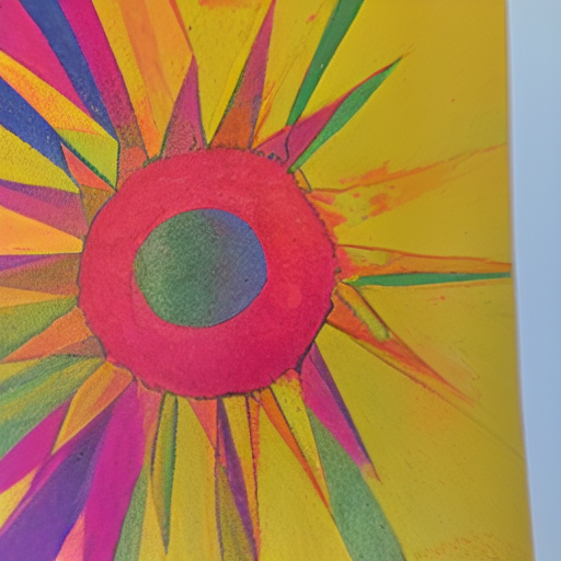
Now we have some theory under our belts, let’s end with two more examples. Below are the results for the prompt ‘dove in the style of brian_wildsmith’. In this series of results, the classifier guidance scale ranges from 0 to 20, increasing in increments of $0.02s$, an order of magnitude smaller than in the sequences above.

At 14 frames per second, it takes about 4 seconds to reach $s=1$. At 4s, the frame is not discernibly a bird, but is just before the turning point at which a bird sharply emerges. This is when the score function is

That is, at $s=1$ the score function is just the conditional denoising model score function – the function we wanted to improve on by introducing classifier, and then classifier-free, guidance. Prior to this point, the images resemble a portrait of a woman: not noise, but not an image that is conditioned on the prompt either. There is another jump in form 16 seconds in, which is when $s=4$. Beyond this, some more Wildsmith-like detail is added, but in general $s>10$ yields minor variations on the result with no particular improvement in quality.

Finally, a tree in the style of Brian Wildsmith. As before, the prompted image emerges a little after $s=1$ (4 seconds in), and there is a long tail of minor variations as $s>4$.

Textual inversion for bias reduction

Finally, I wanted to flag a use case of textual inversion that I haven’t seen discussed beyond the original paper by Gal et al. It is well known that generative models reproduce the biases of their training data. For instance, the prompts ‘doctor’ and ‘scientist’ disproportionately produce images that resemble men. This reflects biases in the kind of images that are uploaded to image hosting sites where the training data is collected from.

When DALL-E2 was first released, this bias recieved a lot of attention and OpenAI scrambled to release a patch that would force the model to produce more diverse images. The first pass solution was surprisingly hacky. It consisted of silently adding a keyword from a list of minority groups (such as ‘female’, ‘black’) to the prompt, as users quickly discovered by prompting the model with “A doctor holding a sign that says”, and observing the keyword printed on the sign in the generated image. This phenomenon isn’t reproducible in current versions, so clearly OpenAI have a more robust solution now. One solution would be to fix the training set. But retraining is computationally expensive.

As the authors of the textual inversion paper suggest, we can use the technique to update a trained model’s understanding of words already in its vocabulary. Rather than using a novel token, as we do when adding a style or object to the model’s vocabulary, we overwrite the embedding of an existing token, training on a small, curated set of images.

The compute budget to do this is negligible relative to training the base model. My textual inversion above ran in about 4 hours on an unspectacular GeForce GTX 1080, whereas the initial training of stable diffusion was 150,000 GPU hours on the considerably more FLOP-heavy A100. This suggests that textual inversion is an elegant and practical tool in the toolbelt to use in countering bias.

References

Ho, J. and Salimans, T. Classifier-free diffusion guidance, In NeurIPS 2021 Workshop on Deep Generative Models and Downstream Applications, preprint https://arxiv.org/abs/2207.12598 2021

Gal, R, Alaluf Y., Atzmon Y., Patashnik O., Bermano A, Chechik G., and Cohen-Or D., An Image is Worth One Word: Personalizing Text-to-Image Generation using Textual Inversion, preprint https://arxiv.org/abs/2208.01618 2022

Nichol, A., Dhariwal, P., Ramesh, A., Shyam, P., Mishkin, P., McGrew, B., Sutskever, I., Chen, M., GLIDE: Towards Photorealistic Image Generation and Editing with Text-Guided Diffusion Models, preprint https://arxiv.org/abs/2112.10741 2022